Topic Modeling with BERTopic and DataMapPlot

Photo by Daniel Kuruvilla on Unsplash

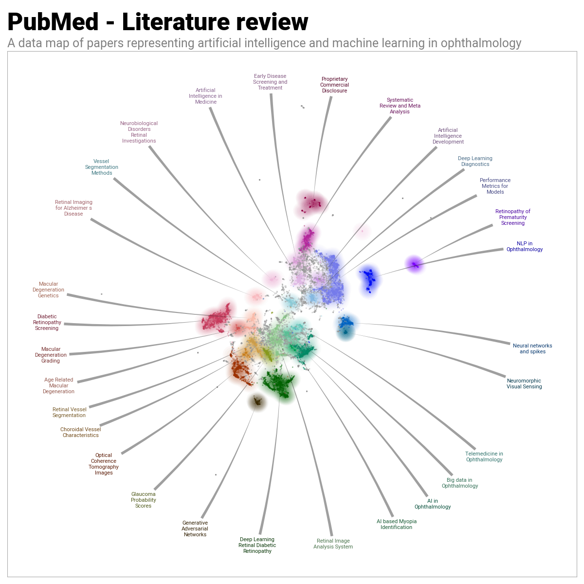
Let me first get straight to the final visualization that this article will go on to create. For the dataset, I ran the following as a PubMed advanced query on 2023/12/28.

(
    (
        "machine learning"[Title/Abstract] OR "artificial intelligence"[Title/Abstract] OR "deep learning"[Title/Abstract]
    ) AND
    (
        "ophthalmology"[Title/Abstract] OR "retina"[Title/Abstract]
    )
)

And by using BERTopic and DataMapPlot, I was able to create the following topic representation.

Introduction

I gave a talk at the biannual Congreso Internacional de Oftalmología Pediátrica, in Puerto Vallarta, México recently. My presentation, entitled “Chatbots in Ophthalmology: The future of patient care?” discussed how greatly the latest generation of large language models had influenced the machine learning community. In turn, my presentation highlighted how so many business domains have already been impacted by the rising complexity and capability of such artificial intelligence innovations. And thus how it would only be a matter of time before even highly domain specific industries such as ophthalmology were likely to also see changes.

The presentation began with an overview of how artificial intelligence is already playing a role in the ophthalmology domain. In particular, I conducted a literature review using the PubMed National Library of Medicine with the following advanced search query:

(
    (
        "machine learning"[Title/Abstract] OR "artificial intelligence"[Title/Abstract] OR "deep learning"[Title/Abstract]
    ) AND
    (
        "ophthalmology"[Title/Abstract] OR "retina"[Title/Abstract]
    )
)

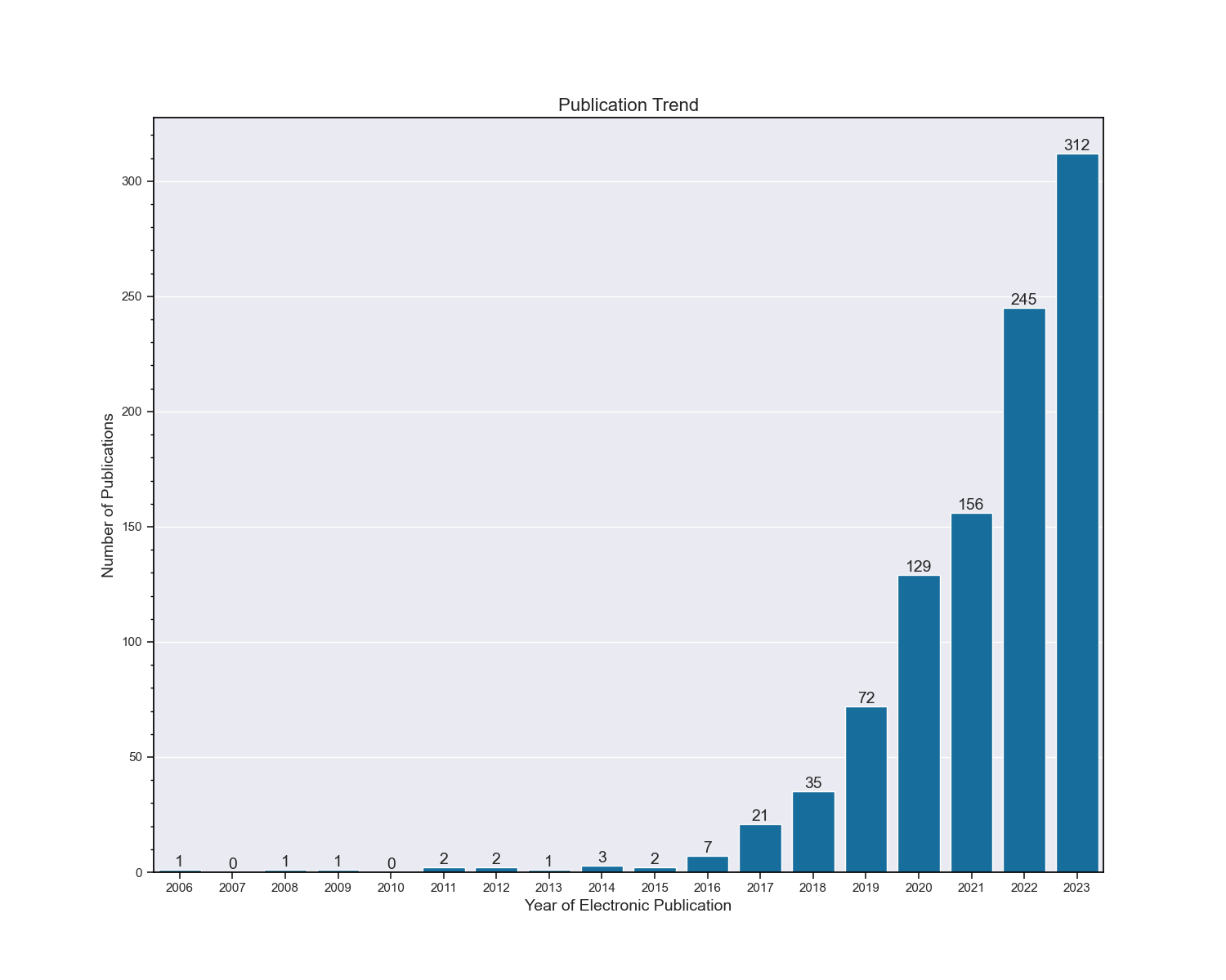
This returned just over 1,200 papers. The trend in electronic publication data is shown in the following figure. Notice in particular the significant increase in the number of publications from 2017/2018 onwards, coinciding with the introduction of the Convolutional Neural Network (CNN) design, other neural network designs such as U-Net (for image medical image segmentation), and indeed the invention of transformer architecture based large language models such as BERT.

However, clearly these research papers embody so much more information about exactly how artificial intelligence has begun to influence ophthalmology. It seemed clear that this would be an excellent candidate for a topic modeling exercise.

Furthermore, as is almost always the case in data science and machine learning, it’s much easier to understand exactly what’s going on when we have some form of data visualization that we can refer to. And so, perhaps I could produce a visualization that efficiently reflected the themes and topics that my topic modeling exercise revealed.

Topic Modeling

Topic modeling is a form of text analysis used in natural language processing (NLP) and machine learning that identifies patterns and themes across a collection of documents. Essentially, it is a method for uncovering the underlying topics or concepts present in a large body of text.

Discovering Hidden Themes: Topic modeling algorithms sift through unstructured text data (like articles, emails, social media posts) to find recurring patterns of words. These patterns are interpreted as topics.

Clustering Similar Content: Instead of reading each document individually, topic modeling groups documents based on similarities in their content. For instance, in a set of news articles, it might find clusters of articles about politics, sports, or finance.

Dimensionality Reduction: It usually helps the interpretation (and visualization) of topic modeling to reduce the complexity of the data (large texts) into more manageable clusters or topics. This makes it easier to process and analyze large datasets.

Unsupervised Learning: Most topic modeling techniques, like Latent Dirichlet Allocation (LDA), are examples of unsupervised learning, where the algorithm identifies patterns without any prior labeling of the data.

Interpreting Topics: The output of a topic model is typically a list of topics, each represented by a cluster of words. Interpreting these topics usually requires human judgment, as the algorithm only knows about word frequencies, not the meaning of the words. Of course, as we’ll come to see, BERTopic allows us to introduce a large language model into our pipeline and have it interpret the topics for us automatically.

BERTopic

For the topic modeling in this article, I used the excellent BERTopic as developed by Maarten Grootendorst. The BERTopic library is in some sense “constructed” over six different modules:

1. Embeddings.
2. Dimensionality reduction.
3. Clustering.
4. Tokenizer.
5. Weighting scheme.
6. Representation tuning (optional).

Embedding documents

Embedding documents involves converting textual data into numerical form. If we imagine each document as a mini-universe of words, then, when we “embed” a document, we’re essentially creating a map of this universe in a way that computers can understand and process. The default method for achieving this in BERTopic is the sentence-transformers framework. I used the specific model paraphrase-multilingual-MiniLM-L12-v2.

from sentence_transformers import SentenceTransformer

embedding_model = SentenceTransformer("all-mpnet-base-v2")

embeddings = embedding_model.encode(docs)

Dimensionality reduction

Once you have created numerical representations of your documents, you usually find that you’ve created a dataset with a very high dimensionality. It is crucial to reduce this high dimensionality to avoid the “curse of dimensionality” phenomenon that typically effects the clustering process (which follows next). But also, it’s important to be keep the number of dimensions in mind throughout the pipeline to ensure that ultimately we can produce a visualization in either two or three dimensions (for our publication). Various techniques, such as Principal Component Analysis (PCA), have been developed to reduce dimensions while retaining essential data characteristics. However, BERTopic uses Uniform Manifold Approximation and Projection (UMAP) by default. UMAP is particularly effective because it manages to preserve both local and global structures within the dataset during dimensionality reduction. This preservation is key, as it retains vital information that enables the formation of clusters comprising documents with similar semantic meanings.

from umap import UMAP

umap_model = UMAP(
    # The size of local neighborhood (in terms of number of neighboring sample points) used for
    # manifold approximation.
    # Larger values result in more global views of the manifold, while smaller values result in
    # more local data being preserved. In general values should be in the range 2 to 100.
    n_neighbors=15,

    # The dimension of the space to embed into.
    # This defaults to 2 to provide easy visualization, but can reasonably be set to any
    # integer value in the range 2 to 100.
    n_components=5,

    min_dist=0.0,
    metric='cosine',
    random_state=42  # For reproducibility - to prevent stochastic behaviour of UMAP.
)

Clustering

The default clustering technique used by BERTopic is HDBSCAN, a density-based clustering method. This technique excels at detecting clusters of varying shapes and can also pinpoint outliers. By not coercing documents into unsuitable clusters, we enhance the quality of our topic representations, minimizing noise and improving clarity.

from hdbscan import HDBSCAN

hdbscan_model = HDBSCAN(
    # Control the number of topics with this parameter.
    # The minimum size of clusters; single linkage splits that contain fewer points than
    # this will be considered points "falling out" of a cluster rather than a cluster splitting
    # into two new clusters.
    min_cluster_size=49,

    metric='euclidean',
    cluster_selection_method='eom',
    prediction_data=True
)

Tokenization

To tokenize our dataset of documents, BERTopic uses the CountVectorizer implementation within sklearn.feature_extraction.text. This effectively gives us a bag-of-words, sparse representation, of the counts of words in our collection of text documents. That is, a matrix of token counts. As stated in the BERTopic documentation, the bag-of-words representation is created on a cluster level rather than a document level. This distinction is important as we are interested in words on a topic level (i.e., cluster level). By using a bag-of-words representation, no assumption is made concerning the structure of the clusters. Moreover, the bag-of-words representation is L1-normalized to account for clusters that have different sizes.

from sklearn.feature_extraction.text import CountVectorizer

vectorizer_model = CountVectorizer(
    ngram_range=(1, 6),
    stop_words=spacy_stop_words,
    analyzer="word",

    # Ignore terms that have a document frequency strictly lower than the given threshold.
    min_df=1,
)

Weighting scheme

This minimum final step (since the tuning of the topic representations is optional) is used to get an accurate representation of the topics present within the bag-of-words sparse matrix created in the previous step. The BERTopic framework uses a class-based TF-IDF feature, developed also by Maarten Grootendorst. He describes the derivation of c-TF-IDF in his website article here. In short, c-TF-IDF can best be described as the TF-IDF formula adopted for multiple classes by joining all documents per class. Thus, c-TF-IDF is used in the context of BERTopic to generate features from textual documents, based on the class they are in i.e. answering the question “what are the most (or top ‘x’) informative words per class?”

from bertopic.vectorizers import ClassTfidfTransformer

# We can choose any number of seed words for which we want their representation
# to be strengthen. We increase the importance of these words as we want them to be more
# likely to end up in the topic representations.
ctfidf_model = ClassTfidfTransformer(
    seed_words=domain_specific_terms,
    seed_multiplier=2
)

Representation tuning

At this point we have generated a set of words that describe our collection of documents i.e. topic representations. However, optionally, we can as a final step, further refine these topics using advanced tools and techniques such as large language models (GPT, T5, etc.), the KeyBERT framework, and the spaCy natural language processing library. Thus, the initial c-TF-IDF topics are considered preliminary, featuring keywords and key documents that allow for further refinement. This approach is particularly beneficial as it enables fine-tuning on a select number of representative documents, significantly reducing the computational load for large models. Consequently, utilizing substantial language models like GPT and T5 in production becomes more practical, often consuming less time than the processes of dimensionality reduction and clustering.

from pathlib import Path

filename_llm = "openhermes-2.5-mistral-7b.Q4_K_M.gguf"
if Path(filename_llm).is_file():
    print(f"Model {filename_llm} exists.")

else:
    url = 'https://huggingface.co/TheBloke/OpenHermes-2.5-Mistral-7B-GGUF/resolve/main/openhermes-2.5-mistral-7b.Q4_K_M.gguf'
    filename_llm = wget.download(url)
    print(f"Model {filename_llm} downloaded.")

from llama_cpp import Llama

# Use llama.cpp to load in a Quantized LLM.
llm = Llama(
    model_path=filename_llm,
    n_gpu_layers=-1,
    n_ctx=4096,
    stop=["Q:", "\n"]
)

from bertopic.representation import KeyBERTInspired, LlamaCPP, MaximalMarginalRelevance, PartOfSpeech

prompt = """Q:
I have a topic that contains the following documents:
[DOCUMENTS]

The topic is described by the following keywords: '[KEYWORDS]'.

Based on the above information, can you give a short label of the topic of at most 5 words?
A:
"""

# Create multiple representations of each topic that BERTopic creates.
# This way when you do e.g. "display(topic_model.get_topic_info()[1:11])" you
# can compare and contrast the different representations of the topics.
# Later on use "topic_model.get_topic_info()" to access all the representations.
representation_model = {
    "LLM": LlamaCPP(llm, prompt=prompt),  # The main pipeline is defined with the "main" key.
    "KeyBERT": KeyBERTInspired(),
    "Aspect1": PartOfSpeech("en_core_web_trf"),
    "Aspect2": [KeyBERTInspired(top_n_words=30), MaximalMarginalRelevance(diversity=.5)],
}

Application of BERTopic

With the above steps completed it is a simple matter to combine the different modular components into the BERTopic framework, so that it may calculate and output the topic representations. In doing so BERTopic also identifies for us which documents contribute to a particular topic allowing us to then calculate the percentage share and cumulative share of documents belonging to a particular topic.

topic_model = BERTopic(
  language="english",

  # Pipeline models.
  embedding_model=embedding_model,            # Step 1 - Extract embeddings.
  umap_model=umap_model,                      # Step 2 - UMAP model.
  hdbscan_model=hdbscan_model,                # Step 3 - Cluster reduced embeddings.
  vectorizer_model=vectorizer_model,          # Step 4 - Tokenize topics.
  ctfidf_model=ctfidf_model,                  # Step 5 - Strengthen topics.
  representation_model=representation_model,  # Step 6 - Label topics.

  # Hyperparameters.
  top_n_words=10,
  verbose=True,

  # Calculate the probabilities of all topics per document instead of
  # the probability of the assigned topic per document.
  # This could slow down the extraction of topics if you have many documents (> 100_000).
  # NOTE: If false you cannot use the corresponding visualization method
  #       visualize_probabilities.
  # NOTE: This is an approximation of topic probabilities as used
  #       in HDBSCAN and not an exact representation.
  calculate_probabilities=True,
)

topics, probs = topic_model.fit_transform(
    docs,
    embeddings,
)

Visualization

The BERTopic framework provides built-in visualization tools that allow you to better understand the topics the model has generated. Given the subjective (and stochastic) nature of the various stages in creating the topic representations these visualizations prove invaluable when it comes to tweaking the model to your particular data set.

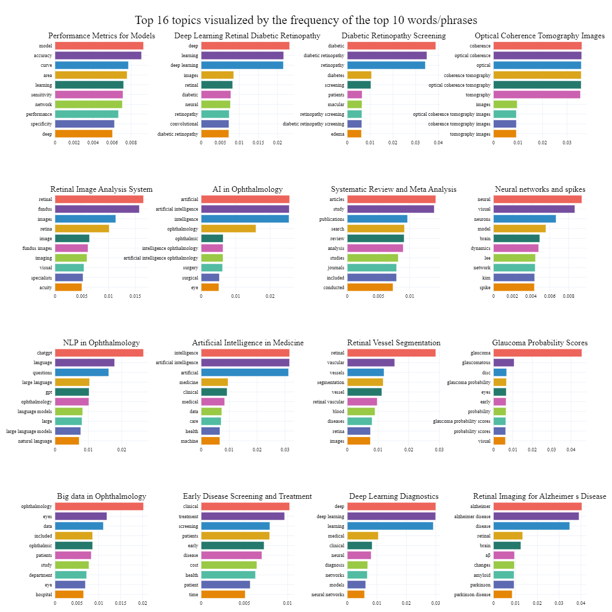
First, a barchart representation of the first 16 topics identified by BERTopic.

import plotly.express as px

top_n_topics = 16
n_words = 10

# 'fig_barchart' is a plotly figure.
fig_barchart = topic_model.visualize_barchart(
    top_n_topics = top_n_topics,  # Only select the top n most frequent topics.
    n_words = n_words,            # Number of words to show in a topic.
    custom_labels=True,          # Whether to use custom topic labels that were defined using topic_model.set_topic_labels.
    title=f"Top {top_n_topics} topics visualized by the frequency of the top {n_words} words",
    width=300,
    height=300,
)

fig_barchart.update_layout(
    # Adjust left, right, top, bottom margin of the overall figure.
    margin=dict(l=20, r=50, t=80, b=20),

    plot_bgcolor='rgba(0,0,0,0)',         # Set background color (transparent in this example).

    title={
        'text': f"Top {top_n_topics} topics visualized by the frequency of the top {n_words} words/phrases",
        'y':0.975,
        'x':0.5,
        'xanchor': 'center',
        'yanchor': 'top',
        'font': dict(
            family="Roboto Black",
            size=24,
            color="#000000"
        )
    },

    font=dict(
        family="Roboto",
        size=10,
        color="#000000"
    ),
)

color_sequence = px.colors.qualitative.Vivid  # Choose a color sequence.
fig_barchart.update_traces(marker_color=color_sequence)

# Show the updated figure
fig_barchart.show()

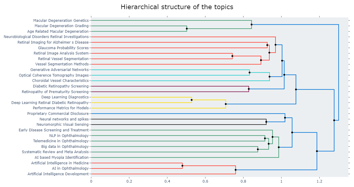
Then, a visualization of the hierarchical structure of the topics found. Here, a Ward linkage function was used to perform the hierarchical clustering based on the cosine distance matrix between topic embeddings.

from scipy.cluster import hierarchy as sch

linkage_function = lambda x: sch.linkage(x, 'ward', optimal_ordering=True)

# Extract hierarchical topics and their representations.
# A dataframe that contains a hierarchy of topics represented by their parents and their children.
hierarchical_topics: pd.DataFrame = topic_model.hierarchical_topics(docs, linkage_function=linkage_function)

fig = topic_model.visualize_hierarchy(
    # 'str' the orientation of the figure. Either 'left' or 'bottom'.
    orientation='left',

    # 'list[int]' a selection of topics to visualize.
    topics=None,

    # 'int' only select the top n most frequent topics to visualize.
    top_n_topics=None,

    # 'pd.DataFrame' a dataframe that contains a hierarchy of topics represented by their
    # parents and their children.
    # NOTE: The hierarchical topic names are only visualized if both 'topics' and 'top_n_topics' are not set.
    hierarchical_topics=hierarchical_topics,

    # Whether to use custom topic labels that were defined using 'topic_model.set_topic_labels'.
    custom_labels=True,

    width=1200,
    height=1000,
)

fig.update_layout(
    # Adjust left, right, top, bottom margin of the overall figure.
    margin=dict(l=20, r=20, t=60, b=20),

    title={
        'text': "Hierarchical structure of the topics",
        'y':0.975,
        'x':0.5,
        'xanchor': 'center',
        'yanchor': 'top',
        'font': dict(
            size=22,
            color="#000000"
        )
    },
)

fig.show()

Separately I used the DataMapPlot library to create a labeled map of the topics, as represented by clusters of points in two-dimensional space.

import datamapplot
import matplotlib.pyplot as plt

# Run the visualization
datamapplot.create_plot(
    reduced_embeddings,
    all_labels,

    use_medoids=True,

    # Follows matplotlib’s 'figsize' convention.
    # The actual size of the resulting plot (in pixels) will depend on the dots per inch (DPI)
    # setting in matplotlib.
    # By default that is set to 100 dots per inch for the standard backend, but it can vary.
    figsize=(12, 12),
    # If you really wish to have explicit control of the size of the resulting plot in pixels.
    dpi=100,

    title="PubMed - Literature review",
    sub_title="A data map of papers representing artificial intelligence and machine learning in ophthalmology",
    # Universally set a font family for the plot.
    fontfamily="Roboto",

    # Takes a dictionary of keyword arguments that is passed through to
    # matplotlib’s 'title' 'fontdict' arguments.
    title_keywords={
        "fontsize":36,
        "fontfamily":"Roboto Black"
    },
    # Takes a dictionary of keyword arguments that is passed through to
    # matplotlib’s 'suptitle' 'fontdict' arguments.
    sub_title_keywords={
        "fontsize":18,
    },

    # Takes a list of text labels to be highlighted.
    # Note: these labels need to match the exact text from your labels array that you are passing in.
    highlight_labels=[
        "Retinopathy Prematurity Screening",
    ],
    # Takes a dictionary of keyword arguments to be applied when styling the labels.
    highlight_label_keywords={
        "fontsize": 12,
        "fontweight": "bold",
        "bbox": {"boxstyle":"round"}
    },

    # By default DataMapPlot tries to automatically choose a size for the text that will allow
    # all the labels to be laid out well with no overlapping text. The layout algorithm will try
    # to accommodate the size of the text you specify here.
    label_font_size=8,
    label_wrap_width=16,
    label_linespacing=1.25,
    # Default is 1.5. Generally, the values of 1.0 and 2.0 are the extremes.
    # With 1.0 you will have more labels at the top and bottom.
    # With 2.0 you will have more labels on the left and right.
    label_direction_bias=1.3,
    # Controls how large the margin is around the exact bounding box of a label, which is the
    # bounding box used by the algorithm for collision/overlap detection.
    # The default is 1.0, which means the margin is the same size as the label itself.
    # Generally, the fewer labels you have the larger you can make the margin.
    label_margin_factor=2.0,
    # Labels are placed in rings around the core data map. This controls the starting radius for
    # the first ring. Note: you need to provide a radius in data coordinates from the center of the
    # data map.
    # The defaul is selected from the data itself, based on the distance from the center of the
    # most outlying points. Experiment and let the DataMapPlot algoritm try to clean it up.
    label_base_radius=15.0,

    # By default anything over 100,000 points uses datashader to create the scatterplot, while
    # plots with fewer points use matplotlib’s scatterplot.
    # If DataMapPlot is using datashader then the point-size should be an integer,
    # say 0, 1, 2, and possibly 3 at most. If however you are matplotlib scatterplot mode then you
    # have a lot more flexibility in the point-size you can use - and in general larger values will
    # be required. Experiment and see what works best.
    point_size=4,

    # Market type. There is only support if you are in matplotlib's scatterplot mode.
    # https://matplotlib.org/stable/api/markers_api.html
    marker_type="o",

    arrowprops={
        "arrowstyle":"wedge,tail_width=0.5",
        "connectionstyle":"arc3,rad=0.05",
        "linewidth":0,
        "fc":"#33333377"
    },

    add_glow=True,
    # Takes a dictionary of keywords that are passed to the 'add_glow_to_scatterplot' function.
    glow_keywords={
        "kernel_bandwidth": 0.75,  # controls how wide the glow spreads.
        "kernel": "cosine",        # controls the kernel type. Default is "gaussian". See https://scikit-learn.org/stable/modules/density.html#kernel-density.
        "n_levels": 32,            # controls how many "levels" there are in the contour plot.
        "max_alpha": 0.9,          # controls the translucency of the glow.
    },

    darkmode=False,
)

plt.tight_layout()

# Save the plot as a PDF, png, and svg file.
plt.savefig('plot_datamapplot.pdf')
plt.savefig('plot_datamapplot.png')
plt.savefig('plot_datamapplot.svg')

Concluding Points

One crucial piece missing from the above discussion is the subtlety that goes into reading in the research paper abstracts, cleaning them, and preparing them for the BERTopic framework. Generally the approach needs to be hands-off as the embedding models are sufficiently sophisticated to be able to discern individual sentences from the abstracts. Thus, applying too much cleaning (e.g. lemmatization, lower-case conversion, etc.) can sometimes hinder the embedding model.

Nonetheless, I think it’s clear that the topics and themes identified by BERTopic are exactly what you would expect from a literature review of the abstracts of research papers covering the search query of artificial intelligence and ophthalmology. In particular, given that this work was completed for the Congreso Internacional de Oftalmología Pediátrica it’s pleasing to see the topic “Retinopathy of Prematurity” represented. In addition, notice how “NLP in Opthalmology” is also represented; perhaps large language models have already appeared in this pediatric ophthalmology domain?!