Loading data into Google Colab

Photo by Mike van den Bos on Unsplash

Introduction

Google Colab (or Colaboratory) is a modern cloud-based runtime environment that gives individuals and teams the ability to work together on coding, data science and machine learning problems with shared access to data, state of the art GPU’s and TPU’s, and industry standard libraries. You are provided with an executable document, i.e. a notebook much like a Jupyter Notebook, that allows both code and markdown to be written and executed, and your results visualized. That is to say, Google Colab is a complete a working environment for teams to prototype and execute Python, HTML, and LaTeX in a cooperative manner. In addition, Google Colab allows you to share your work within the Google Drive (Cloud) environment or indeed through GitHub.

Just as with a Jupyter notebook, a Google Colab notebook is composed of cells, each of which can contain code, text, images, etc. Colab connects your notebook to a cloud-based, Google hosted, runtime; meaning you can execute Python code without any required setup on your own machine. Additional code cells are executed using that same runtime, resulting in an interactive coding experience in which you can use any of the functionality that Python offers.

Google Colab also comes complete with a built-in library of code snippets meaning you can easily insert code to solve the most common of computing problems. And Colab also supports many 3rd party Python libraries as well.

Colab notebooks can be shared just like any other Google Document - thus the ability to include text cells in your notebook allows you to create a narrative around your code, just like a shared laboratory workbook. Text cells are formatted using Markdown, again just as with Jupyter notebooks, allowing you to add headings, paragraphs, lists, and even mathematical formulae. The analogy to a Jupyter notebook is completed by being able to save your work as a .ipynb file so it can be viewed and executed later, say, locally on your machine, or in JupyterLab, or any other compatible framework.

Examples of projects shared by other teams can be found at Google’s AI Hub (the Seedbank project). See also the documentation for many other examples of what is available in Seedbank.

In this article we’ll take a look at the many different ways you can get data into your Colab notebook, whether from your local machine, or elsewhere in the cloud, in order to get started on your project.

Getting Setup with Colab in Google Drive

Google Colab is based around Google Drive, the personal cloud storage and file sharing platform hosted by Google. If you don’t already have an account on Google Drive, simply head to the sign-in page to create an account.

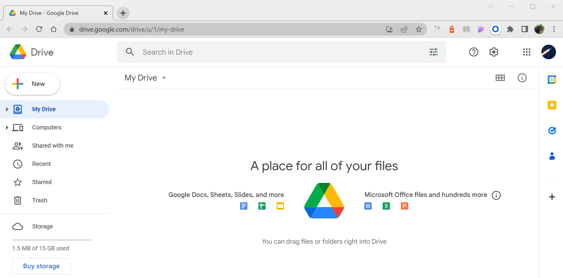
From your Drive homepage selecting the “New” button allows you to create different types of files - typically from the category of office productivity, such as Google Docs, Google Sheets, and Google Slides. But in addition, if you select the “More” option you’ll see which additional types of documents are available to you.

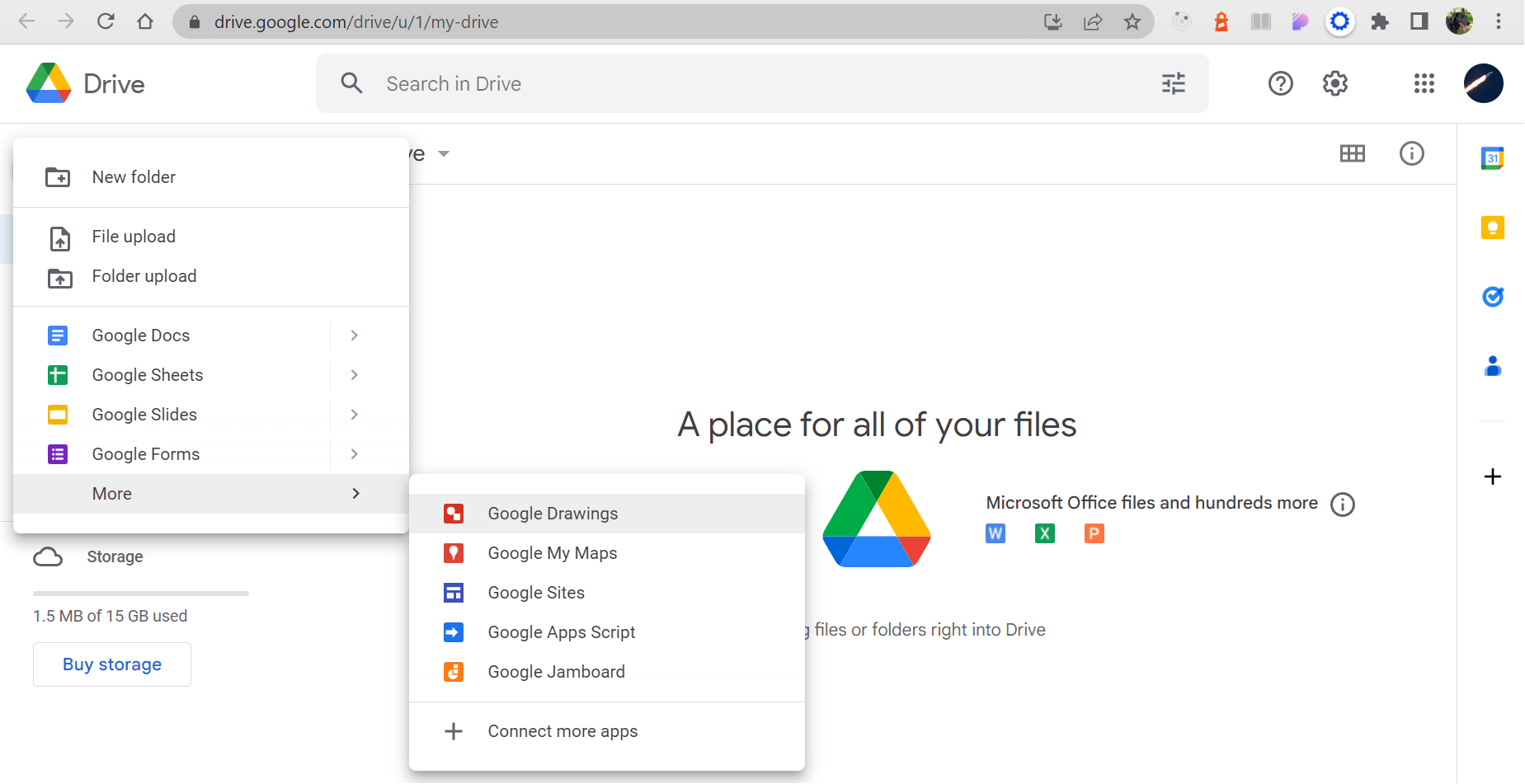
If you’ve worked with Google Colab before you should see “Colaboratory” as an option within the “More” option just mentioned. However, if this is your first time creating a blank notebook it’s possible the “Colaboratory” button isn’t shown at all. In which case, click on the “Connect more apps” option and in the window that pops-up select (or search for) “Colaboratory”. This will give you the option to install Google Colab within your Google Drive environment.

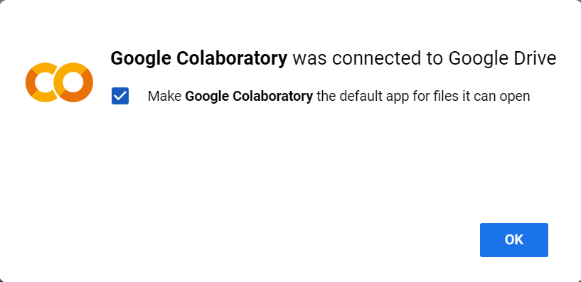
And so you should now have the “Colaboratory” option available to you via the “New” menu as previously mentioned.

Create a New Notebook

Selecting “Colaboratory” from the “New” menu creates and opens a new, blank notebook for you.

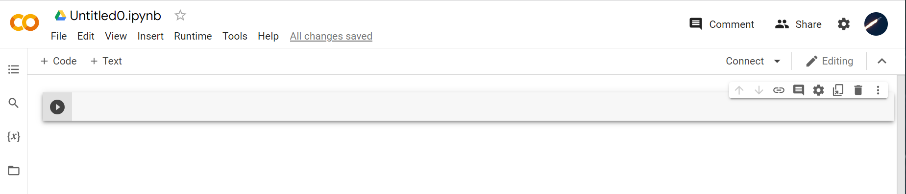
As I’ve mentioned above, you can think of and use this environment in pretty much the same way you would a locally hosted Jupyter Notebook file. So for example you can change the default filename, you can enter code and Markdown into the cells, and you can create new cells as and when they are needed.

Just note, it’s a good idea to double check the runtime you are using. Do this by selecting “Runtime” from the navigation menu at the top of the screen, and then selecting “Change runtime type”.

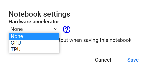
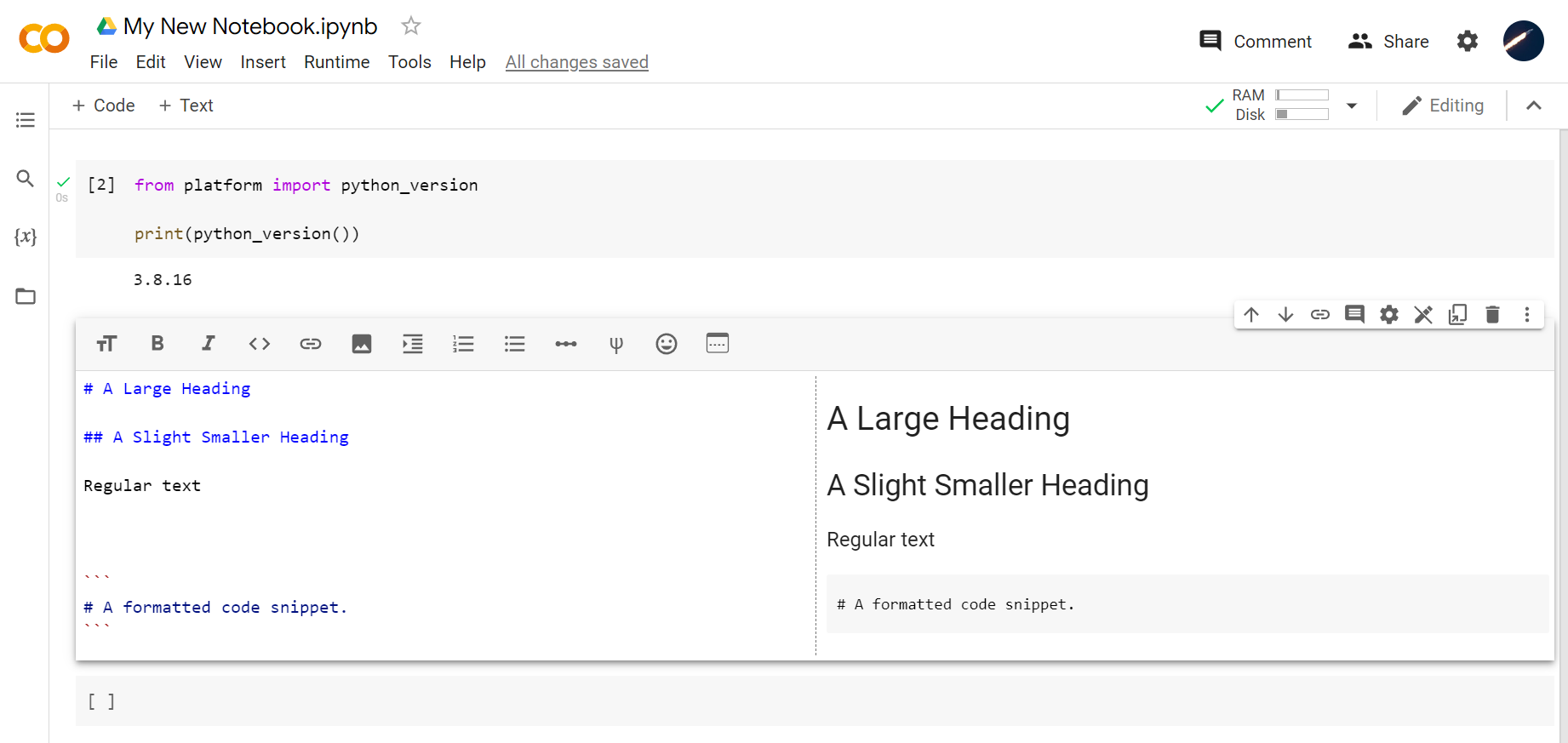
Here you’ll see how straightforward it is to select a GPU or TPU runtime. Choosing “None” implies using a CPU based Python implementation. Try the following code snippet to see which version of Python is being used.

from platform import python_version

print(python_version())

Note that sometimes a GPU or TPU might not be available. This is because these are shared resources. Thus it’s possible that other users, anywhere around the world, might also be using Google Colab. Since we are all sharing these resources if the usage hits the limit of what’s available, then you might not have a GPU or TPU available at the time you need them. It shouldn’t make a difference to the Python code you write of course.

Next, notice that you can create code cells and text cells. The image above shows an example of a code cell, and below we see examples of both code and text cells. In particular we see how text cells allow you to write Markdown, with the left hand side of the cell available for you to input text, and the right hand side showing a preview of what that text will look like once you execute the cell.

Making data available

So, to the focus of this article, making data available in your Colab environment for you to work with.

Using wget

The first method we’re going to look at is simply the classic Linux command wget. As is the case in a regular Jupyter notebook, you can indeed run command line commands in a Google Colab notebook by preceding the command with an exclamation mark.

In the following snippet, we download the “Car Evaluation Data Set” from the University of California, Irvine’s ICS, UCI repository.

!wget https://archive.ics.uci.edu/ml/machine-learning-databases/car/car.data

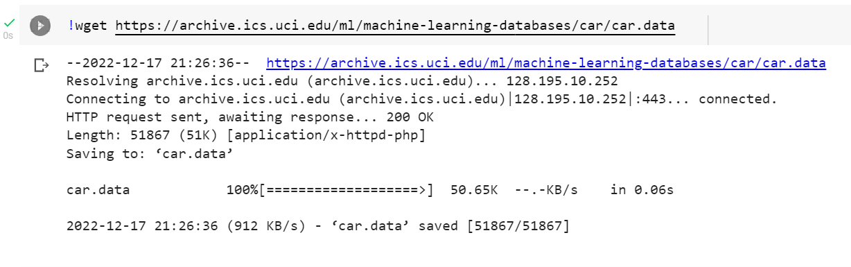
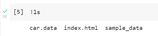
Running the above in a code cell within your Colab notebook downloads the car.data file to the current directory (hosted on Google Cloud). So, for example running !ls in the new code cell shows you where the file is located.

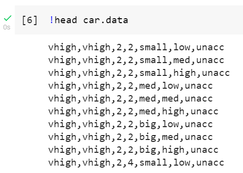
To get a handle on what the data looks like, within car.data, you can run !head car.data, which in particular will tell you whether there is a header row.

Perhaps it would be more familiar to use Python pandas to read in the data file:

import pandas as pd

df_car = pd.read_csv('car.data', header=None)

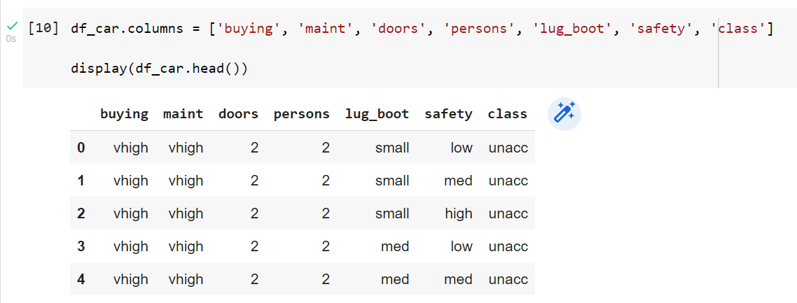
And since we’re using ICS, UCI data, we’re lucky enough to have documentation that describes what the appropriate headers are:

df_car.columns = ['buying', 'maint', 'doors', 'persons', 'lug_boot', 'safety', 'class']

display(df_car.head())

Using tf.keras

The next method involves using the Tensorflow library directly, in particular the Keras api. This method can also be used if your data is available via a url, as was the case above.

This time we’ll use the “Wine” data set, again from ICS, UCI.

First, define the url for the data:

url = 'https://archive.ics.uci.edu/ml/machine-learning-databases/wine/wine.data'

Then install and import the tensorflow library:

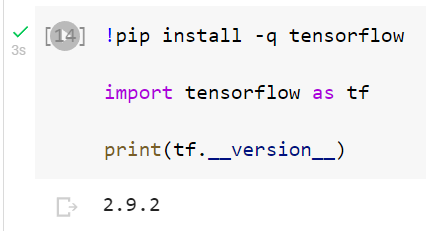
!pip install -q tensorflow

import tensorflow as tf

print(tf.__version__)

Now we call the Keras get_file() function in order to download the data. Here the first argument represents the full path that we want to save the data to - while the second argument represents the source (in this case our url).

tf.keras.utils.get_file('wine.data', url)

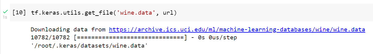
Notice how the data is saved in a default Keras based location, as shown in the output of get_file() being the location 'root/.keras/datasets/wine.data'.

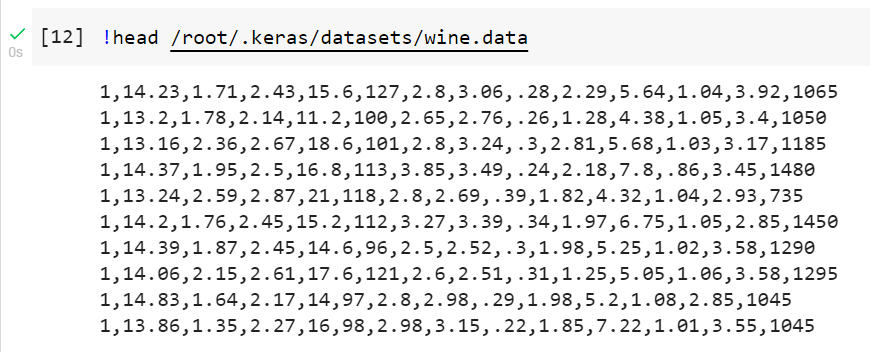
Now, just as we did earlier, we can use the !head /root/.keras/datasets/wine.data to take a quick look at the data - this time ensuring we use the full path to the data.

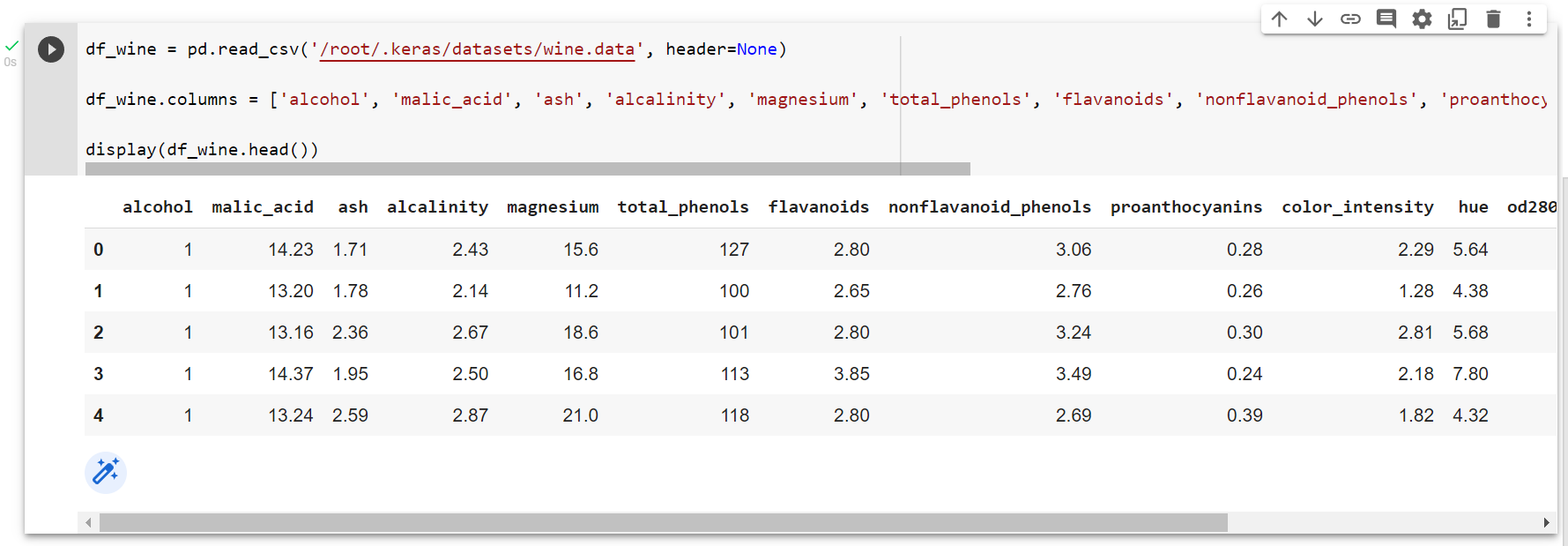
And we import the data into a pandas DataFrame with the appropriate column names.

df_wine = pd.read_csv('/root/.keras/datasets/wine.data', header=None)

df_wine.columns = ['alcohol', 'malic_acid', 'ash', 'alcalinity', 'magnesium', 'total_phenols', 'flavanoids', 'nonflavanoid_phenols', 'proanthocyanins', 'color_intensity', 'hue', 'od280_od315_of_diluted_wines', 'proline', 'class']

display(df_wine.head())

Uploading a local file

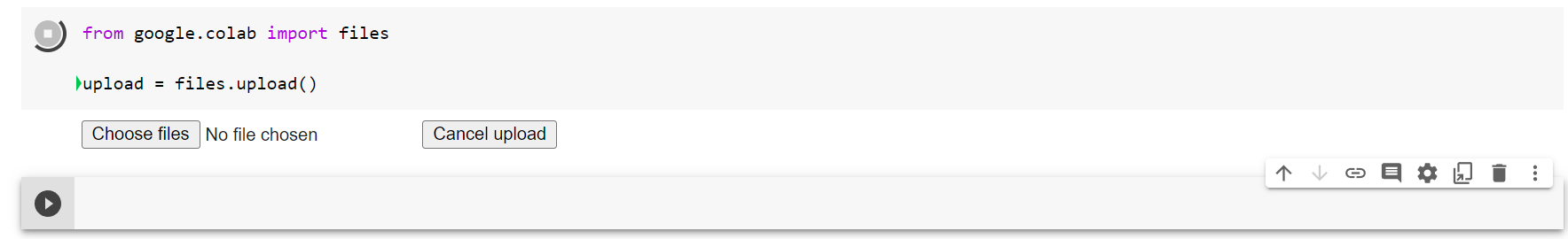
For the third method we’ll upload a file we have stored on our local machine. To do so, we need to run a built-in Colab function from the files module named upload():

from google.colab import files

upload = files.upload()

This will enable a choose file dialog, with which we can select the locally held file we wish to upload.

Here I choose the Adult data set, which I previously downloaded from ICS, UCI.

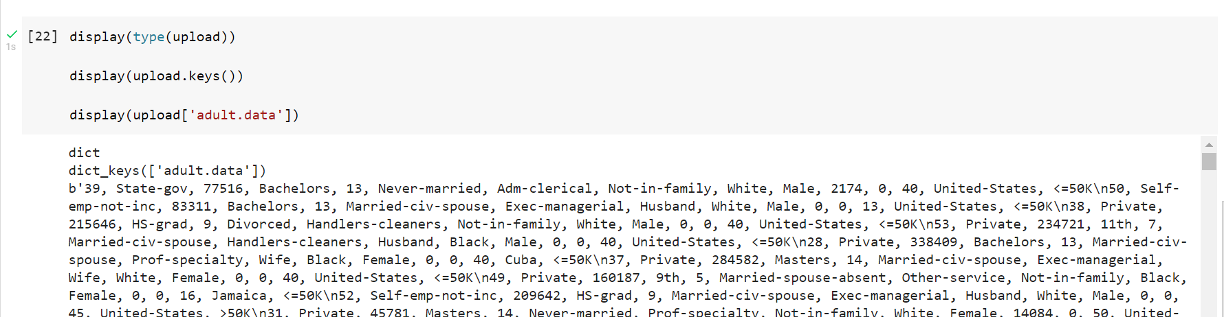
Notice that the upload variable becomes a Python dictionary, with a single key that is the name of the file, and whose value is the actual data content of the file.

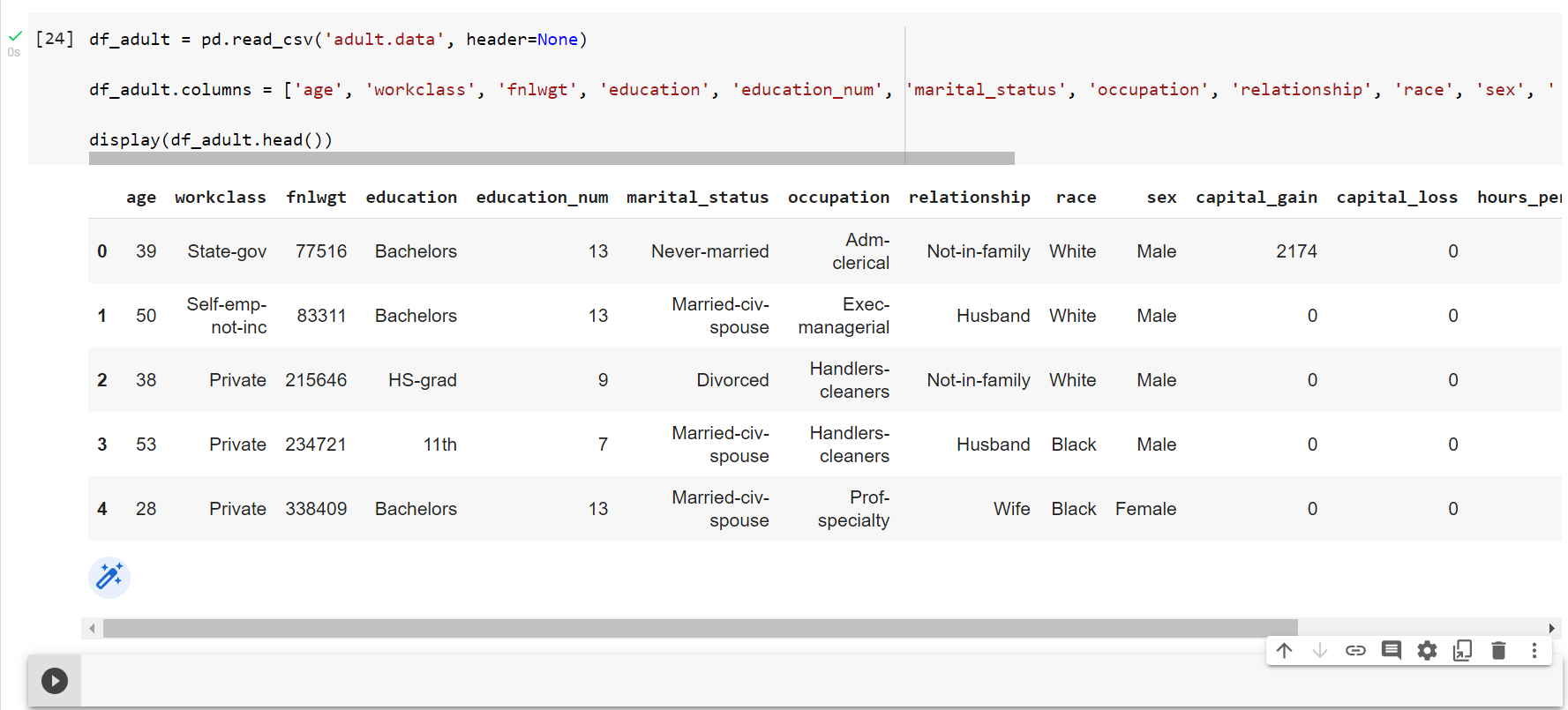
Just as we’ve done in the previous two examples, we’ll read in the file into a pandas DataFrame:

df_adult = pd.read_csv('adult.data', header=None)

df_adult.columns = ['age', 'workclass', 'fnlwgt', 'education', 'education_num', 'marital_status', 'occupation', 'relationship', 'race', 'sex', 'capital_gain', 'capital_loss', 'hours_per_week', 'native_country', 'class']

display(df_adult.head())

Accessing files from our Google Drive

It would be a little strange if we couldn’t access data stored in our own Google Drive, from a Colab notebook that was itself being run within that Drive environment!

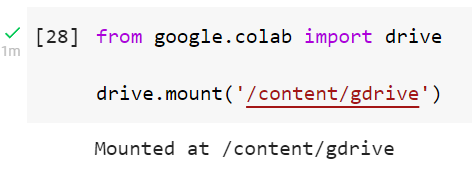
Well, of course, the answer is yes we can; Google Colab provides a built-in function, from the drive module, named mount():

from google.colab import drive

drive.mount('/content/gdrive')

Upon running the above, Google will ask you for permission to see, edit, create and delete files from your Google Drive.

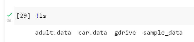
And so if we now run the linux command !ls we’ll see an additional folder named gdrive:

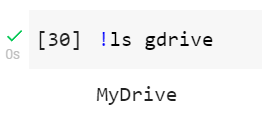
Inside of this folder we see a reference to our own Google Drive location:

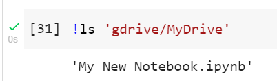
And inside there - sure enough - we find the very same Colab notebook that we are working with:

Thus, assuming you have a data file already uploaded to your Google Drive, it would be a straightforward matter to now read that data into a pandas DataFrame.

Conclusion

So there you have it. There really is nothing to it. The particular method you choose will of course depend on the problem you are working on and the particular source(s) of your data. Good luck!