
Introduction
Clustering is a fundamental technique in data science, machine learning, and applied mathematics. At its core, it provides us a way to uncover hidden structure and patterns in data by grouping similar items — often represented them as vectors — based on how close they are to one another in some feature space.
In this article, I explore the problem of clustering a collection of vectors into meaningful groups, where similarity is typically measured by the distance between pairs of vectors. The focus is on one of the most well-known and widely used clustering methods: the K-Means algorithm. Along the way, I’ll demonstrate typical practical applications and provide Python examples for further illustration.
The Value of Clustering
Clustering is a fundamental and versatile technique used across a wide range of fields—including data science, machine learning, and mathematics—to uncover hidden structure and patterns in data.
In data science, clustering is often used in exploratory data analysis to reveal natural groupings within a dataset. These groupings may not be obvious at first glance, but once identified, can provide critical insights. For example, in a marketing context, clustering can help segment customers based on behaviour or purchasing patterns, making large, unwieldy datasets more manageable—and ultimately more useful. These segments can also improve the performance of downstream machine learning models by focusing them on more coherent subsets of data. Clustering can even help identify noise or anomalies, making it useful for tasks like fraud detection or outlier analysis.
Another important use of clustering is in feature engineering. By assigning each data point to a cluster, we can create new features that encode group membership—features; the group similarities carry meaningful information for predictive models - meaning that has been engineered from the dataset.
In machine learning, clustering algorithms usually fall under the umbrella of unsupervised learning; that is, models that derive their insights from unlabeld data. Since it doesn’t require labeled data, it’s particularly useful in domains where labels are expensive or difficult to obtain. Clustering can serve as a preprocessing step (~ feature engineering) to generate pseudo-labels for semi-supervised learning, or to break a dataset into smaller, more homogeneous distributions that can be modeled independently.
Clustering is also helpful in dimensionality reduction. By summarizing groups of similar data points, it allows us to simplify complex, high-dimensional datasets into more digestible forms (typically with fewer dimensions). This can then aid in visualization and interpretation, especially in domains like image processing (e.g., segmenting images into meaningful regions) or natural language processing (e.g., topic modeling via semantic similarity of sentences). In fact, I used clustering for topic discovery in my presentation, “The Intersection of Artificial Intelligence and Ophthalmology” at XXX Congreso Boliviano de Oftalmología (see my review article here).
Finally, from a mathematical perspective, clustering helps identify geometric and statistical structure in data. It can reveal relationships between points in a metric space or model distributions within data, as in the case of Gaussian Mixture Models, which are often used in fields like population dynamics.
Types of Clustering
Before we get into the detail of the K-Means clustering algorithm lets briefly review some of the other algorithms that are popular within the data science and machine learning community. Each method has its strengths and trade-offs, and the right choice often depends on the shape of your data, the level of noise, and whether or not you know how many clusters to expect.
Hierarchical Clustering
This method builds a hierarchical tree of clusters i.e. a tree-like structure. It can be subdivided into two main types:
- Agglomerative (bottom-up): Starts with each data point as its own cluster and iteratively merges pairs of clusters based on a similarity metric.
- Divisive (top-down): Starts with all points in a single cluster and recursively splits them.
The strengths of hierarchical clustering are that there is no need to predefine the number of clusters. This is advantagous since with a new dataset you may have no reason to choose a certain number of clusters over another - especially if you don’t have specific domain-knowledge.
The weaknesses of hierarchical clustering is it is potentially computationally expensive for large datasets. Although GPU processing may aleviate this, it can still represent a high entry bar for starting your analysis.
DBSCAN
DBSCAN (Density-Based Spatial Clustering of Applications with Noise) is a density-based clustering algorithm that identifies clusters as regions of high data density separated by more sparse regions. Points are classified as core points, border points, or noise based on their neighborhood density.
It’s strength is that it can detect clusters of arbitrary shapes. Also, it handles noise and outliers well. It’s weakness is that it is sensitive to parameter choices and tuning (especially for the eps and min_samples parameters).
Mean Shift Clustering
Mean Shift is a centroid-based algorithm that iteratively shifts candidate centroids towards regions with higher point density. Thus moving centroids toward the mean of the data points, within a defined bandwidth (radius) - effectively shifting toward the “center of mass” of the data within a certain radius.
The strengths of mean shift clustering include being able to find clusters without predefining their number in advance. Again, an advantage when you have no prior (domain) knowledge of what an appropriate number of clusters should be. Also, mean shift clustering works well for non-spherical clusters. The weaknesses include it being computationally intensive and being highly sensitive to bandwidth (radius) selection.
Gaussian Mixture Models
Gaussian Mixture Models (GMM) is a probabilistic model that assumes the data is generated from a mixture of several Gaussian distributions, each representing a cluster. Unlike K-Means, GMM assigns soft cluster memberships to each point i.e. each point has a probability of belonging to each cluster, rather than a hard cluster membership assignment.
Regarding it’s strengths, GMMs are flexible and can handle overlapping clusters and non-spherical shapes. Its weaknesses include it being computationally expensive, and the fact it is sensitive to initialization settings. Also, GMMs may converge to a local optimum rather than global.
Spectral Clustering
Spectral Clustering uses the eigenvalues of a similarity matrix (derived from the graph representation of the data) to reduce dimensionality before applying a clustering algorithm like K-Means. It is particularly effective for non-convex clusters i.e. when clusters are non linearly separable.
Strengths include it being effective for clusters with complex shapes and that it is not limited to linear data separations. It’s weaknesses are that it requires a well-defined, meaningful similarity graph for operation, and that it can be computationally demanding.
OPTICS
OPTICS (Ordering Points To Identify the Clustering Structure) is a density-based algorithm similar to DBSCAN but which is better suited to data with varying densities. It generates an augmented ordering of the dataset so as to then create a reachability plot, which helps visualize the clustering structure.
OPTICS is moore robust than DBSCAN when clustering structure varies in density, but interpreting the reachability plot can be challenging.
Affinity Propagation
This algorithm treats every point as a potential cluster center (i.e., an ‘exemplar’ or ‘repreentative point’) and uses message-passing between points to identify exemplars and define their associated clusters. Unlike K-Means, it does not require the number of clusters to be predefined.
It’s strengths are that it can find clusters of varying sizes, does not require the number of clusters to be specified in advance, and is less sensitive to initialization. It’s weaknesses are that it can be computationally expensive and can sometimes over-fragment the dataset into (too) many small clusters.
BIRCH
BIRCH (Balanced Iterative Reducing and Clustering using Hierarchies) is designed for very large datasets. It incrementally clusters incoming data points by summarizing them using a specialized tree structure called the Clustering Feature Tree.
BIRCH scales well to very large datasets while remaining memory-efficient. However, it assumes the clusters are spherical and so may not perform well with arbitrary or complex cluster shapes.
CURE
CURE (Clustering Using Representatives) identifies clusters by selecting multiple representative points for each cluster, and then shrinks them towards the cluster’s centroid. Doing so dampens the influence of outliers and thus improves robustness against noise.
It handles clusters of varying shapes and sizes better than more traditional centroid-based methods but it is more computationally intensive (than those traditional, simpler methods) for large datasets.
The Goal of Clustering
Suppose that we have
That is to say, each vector has
Part of the task of clustering a collection of vectors is to determine whether or not the vectors can be divided into
Normally we have
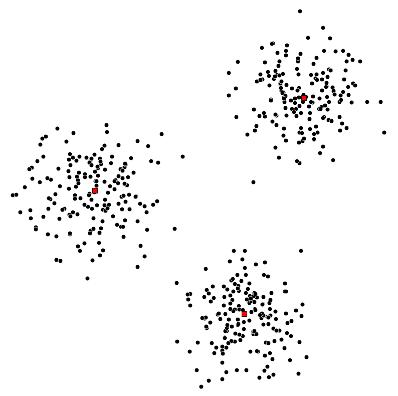
| Toy dataset |
|---|
|
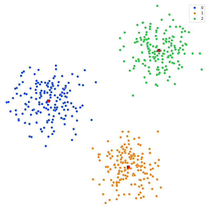
| K-Means clustering |
|---|
|
Illustration of a toy dataset (left) and the result of clustering with k=3 (right) using the Python scikit-learn library - modules make_blobs and KMeans respectively.
The illustration above shows a simple example, with
Note of course that this example is not typical in several ways:
- First, the vectors have dimension
. Clustering any set of 2-vectors is easy - we simply create a scatter plot of our dataset and check visually if the points are clustered, and if so, how many clusters there are. In almost all applications is larger than (and typically, much larger than ), in which case this simple visual method cannot be used. In the more general case, for is larger than , visual inspection cannot replace formal methods like silhouette score or elbow method; again, especially in high-dimensional spaces. - Secondly, the points are very well clustered. In most applications the data will not be as cleanly clustered as in this toy example; data from the real world is usually messy, with several if not many points lying in between clusters.
Even though the above example is not typical, and the best value of
Common applications of clustering
Clustering is widely used across many technical, data-focused fields to find meaningful structure in unlabeled data. Here are some typical applications, each framed in terms of clustering vectors
Topic discovery
Suppose
Patient clustering
Let
Customer market segmentation
Suppose the vector
ZIP or Post Code clustering
Suppose that
Student clustering
Suppose the vector
Survey response clustering
A group of
Weather zones
For each of
Daily energy use patterns
The 24-vectors
Financial sectors
For each of
Clustering Objective
Let’s now formalize the clustering procedure, and introduce a natural measure to quantify the quality of a given clustering.
Specifying the cluster assignments
We specify a clustering of vectors by stating which cluster or group each vector belongs to. We label the groups
- As a simple example with
vectors and groups, means that: is assigned to group . , , and are assigned to group . is assigned to group .
We also describe the clustering by the sets of indices for each group; let
For our simple example above, we have:
Formally, we can express these index sets in terms of the group assignment vector
Group representatives
With each of the groups we associate a group representative n-vector, which we denote
We want each representative to be close to the vectors in its associated group:
Note that
The Clustering Objective
We can now give a single number that we use to judge a choice of clustering, along with a choice of the group representatives.
We define:
which is the mean square distance from the vectors to their associated representatives. This is an “ensemble average” often referred to in statistical mechanics as a measure of the deviation of the position of a particle with respect to a reference position (and often as a function of time such that it can be updated over time). It is the most common measure of the spatial extent of random motion, and can be thought of as measuring the portion of the system “explored” by the random walker.
Note that
An extreme case is
Our choice of clustering objective
- For example, it is possible to use an objective that encourages more balanced groupings.
- But we will stick with this basic (and very common) choice of clustering objective.
The k-Means Algorithm
The two calculations we need to solve
We have two calculations to fulfill:
- Choosing the group assignments.
- Choosing the group representatives.
Both of which are required to minimize
Solving the two calculations
The two choices/calculations we need to make are circular, i.e., each depends on the other. Thus, instead of solving directly we rely on a very old idea in computation … we simply iterate between the two choices.
This means that we repeatedly alternate between updating the group assignments, and then updating the representatives. In each step the objective
Iterating between choosing the group representatives and choosing the group assignments is the celebrated K-Means algorithm for clustering a collection of vectors.
And so (finally!) to the K-Means algorithm
The K-Means algorithm was first proposed in 1957 by Stuart Lloyd, and independently by Hugo Steinhaus. It is sometimes called the Lloyd algorithm. The name “K-Means” has been used since the 1960s.
In pseudocode the algorithm reads like the following:
Repeat until convergence:
- Partition the vectors into k groups. For each vector i=1, …, N, assign x1 to the group associated with the nearest representative.
- Update representatives. For each group j=1, …, k, set zj to be the mean of the vectors in group j.
Regarding convergence, the fact that
However, depending on the initial choice of representatives, the algorithm can, and does, converge to different final partitions, with different objective values.
The K-Means algorithm is a heuristic, which means it cannot guarantee that the partition it finds minimizes our objective
For this reason it is common to run the K-Means algorithm several times, with different initial representatives, and choose the one among them with the smallest
final value of
Let’s create a gif animation to demonstrate the iteration of the K-Means algorithm, as we’ve just defined it. First, create a toy dataset, using the make_blobs module from scikit-learn.
# X - ndarray of shape (n_samples, n_features)
#     The generated samples.

# Generate synthetic data using make_blobs
X, _ = make_blobs(
    # Effectively the number of rows in the matrix X.
    n_samples=500,
    centers=[[-5, 3], [5, -5], [9, 9]],
    # Effectively the number of columns in the matrix X.
    n_features=2,
    cluster_std=2.0,
    random_state=69,
    return_centers=False
)
Then, define a similar target for K-Means clustering, again as we did previous. We expected there to be 3 clusters so we set n_clusters=3. We can set as many iterations as we feel is necessary with max_iter, knowing that in the code below there will be a if clause that looks for convergence. Let’s also define the locations of our centroids. These are initialized to points randomly selected from
# K-Means parameters
n_clusters = 3
max_iter = 10
plot_ranges = [[-9.5, 13.5], [-10, 14]]

np.random.seed(0)

# Randomly select 'n_clusters' unique indices from
# the range [0, len(X)) i.e. to len(X) - 1.
# False ensures that the same point is not selected more than once.
# Thus the 'n_clusters' centroid's intial positions are initialized
# to points randomly selected from X (i.e. taken from the dataset itself).
centroids = X[np.random.choice(len(X), n_clusters, replace=False)]
Initialize a list to store the results of each iteration. And thus store the initial locations of the centroids and the associated initial clustering label groupings.
# Initial assignment of points to the nearest centroid.
# This function computes for each row in 'X', the index of
# the row of 'centroids' which is closest to it.
# The default distance metric used is the Euclidean distance.
initial_labels = pairwise_distances_argmin(X, centroids)
labels_history = [initial_labels]

centroids_history = [centroids.copy()]

# Calculate intial mean square distance.
squared_distances = np.sum((X - centroids[initial_labels]) ** 2, axis=1)
mean_square_distance = np.mean(squared_distances)
print(f"Initial iteration: Mean Square Distance = {mean_square_distance}")
Iterate over the steps we defined in our pseudocode above.
# Iterate the K-Means algorithm based on our pseudocode.
for iteration in range(1, max_iter):
    # Step 1: Assign points to the nearest centroid.
    labels = pairwise_distances_argmin(X, centroids)

    # Step 2: Compute new centroids.
    new_centroids = []
    for i in range(n_clusters):
        points_in_cluster = X[labels == i]
        if len(points_in_cluster) > 0:
            new_centroids.append(points_in_cluster.mean(axis=0))
        else:
            # No points assigned to this cluster, keep the centroid the same.
            new_centroids.append(centroids[i])

    new_centroids = np.array(new_centroids)

    # Calculate mean square distance
    squared_distances = np.sum((X - new_centroids[labels]) ** 2, axis=1)
    mean_square_distance = np.mean(squared_distances)

    # Check for convergence
    if np.allclose(centroids, new_centroids):
        print(f"\nConverged after {len(centroids_history) - 1} iterations.\nThe centroid positions after the {len(centroids_history)} iteration being identical to the previous iteration.")
        break

    print(f"Iteration {iteration}: Mean Square Distance = {mean_square_distance}")

    # Reassign points to the nearest centroid.
    # The new centroids and labels should only be appended to their respective histories if
    # convergence has not been reached. This will prevent the final two entries from being identical.
    labels_history.append(labels)
    centroids_history.append(new_centroids.copy())

    centroids = new_centroids

# Ensure both histories are the same length
try:
    assert len(centroids_history) == len(labels_history)
except AssertionError:
    print(f"centroids_history:\n{centroids_history}\n")
    print(f"labels_history:\n{labels_history}\n")
    raise AssertionError(f"Length of centroids_history ({len(centroids_history)}) and labels_history ({len(labels_history)}) do not match.")
else:
    # Check if the final two entries of 'centroids_history' are identical.
    if np.array_equal(centroids_history[-1], centroids_history[-2]):
        print("The final two entries of 'centroids_history' are identical.")
    # Likewise for 'labels_history'.
    if np.array_equal(labels_history[-1], labels_history[-2]):
        print("The final two entries of 'labels_history' are identical.")
Plot the result, step by step, to a gif.
# Create animation
fig, ax = plt.subplots(figsize=(10, 10))

def init():
    ax.clear()
    ax.set_xlim(plot_ranges[0])
    ax.set_ylim(plot_ranges[1])
    ax.spines['top'].set_visible(False)
    ax.spines['bottom'].set_visible(False)
    ax.spines['left'].set_visible(False)
    ax.spines['right'].set_visible(False)
    ax.xaxis.set_tick_params(labelbottom=False, length=0)
    ax.yaxis.set_tick_params(labelleft=False, length=0)
    return ax,

def update(frame):
    ax.clear()
    sns.scatterplot(
      x=X[:, 0], y=X[:, 1],
      hue=labels_history[frame],
      palette="bright",
      s=40
      ax=ax,
      legend=None
    )
    ax.scatter(
      centroids_history[frame][:, 0], centroids_history[frame][:, 1],
      s=60, c='red', marker='X', edgecolor='black'
    )
    ax.set_xlim(plot_ranges[0])
    ax.set_ylim(plot_ranges[1])
    ax.set_title(f"K-Means Clustering - Iteration {frame + 1}")
    ax.spines['top'].set_visible(False)
    ax.spines['bottom'].set_visible(False)
    ax.spines['left'].set_visible(False)
    ax.spines['right'].set_visible(False)
    ax.xaxis.set_tick_params(labelbottom=False, length=0)
    ax.yaxis.set_tick_params(labelleft=False, length=0)
    return ax,

min_frames = min(len(centroids_history), len(labels_history))

ani = FuncAnimation(
  fig, update, frames=min_frames, init_func=init, blit=False
)

# Save the animation as a GIF.
ani.save(
  "kmeans_clustering_animation.gif", writer="imagemagick", fps=1
)

plt.close(fig)
Giving us the following iterative progress.
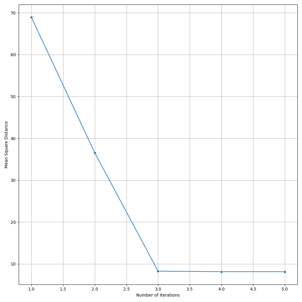
Concluding thoughts
To conclude let us simply remind ourselves that clustering algorithms serve as foundational techniques across the domains data science, machine learning, and mathematics, offering a way to uncover inherent structures and patterns in data. We focused specifically on the K-Means algorithm, it being one of the most popular unsupervised techniques available to the data science community. We then went on to discuss the many different applications of clustering, followed by a walkthrough of the algorithm for K-Means. We finished with an animated gif of the iterative process behind K-Means.
References
- Introduction to Applied Linear Algebra: Vectors, Matrices, and Least Squares, Boyd and Vandenberghe, Cambridge University Press, 2018.
- Pham, D. & Dimov, Stefan & Nguyen, Cuong. (2005). Selection of K in K-means clustering. Proceedings of The Institution of Mechanical Engineers Part C-journal of Mechanical Engineering Science - PROC INST MECH ENG C-J MECH E. 219. 103-119. 10.1243/095440605X8298.
- Wu, J. (2012). Advances in K-means Clustering. Springer Theses. 10.1007/978-3-642-29807-3